
Archive for February, 2020
Prediction-based recommendation in process mining
This post is by Gyunam Park, Scientific Assistant in the Process And Data Science group at RWTH Aachen University. Contact him via email for further inquiries.
Process mining has provided effective techniques to extract in-depth insights into business processes such as process discovery, conformance checking, and enhancement. Nowadays, with the increasing availability of real-time data and sufficient computing power, practitioners are more interested in forward looking techniques whose insights can be used to improve performances and mitigate risks of running process instances.
Research on these forward looking techniques has been actively done in the field of process mining. Predictive business process monitoring is one of those approaches, whose aim is to improve business processes by offering timely information (e.g., remaining time of running instances) that enables proactive and corrective actions.
However, these techniques do not suggest how the predictions are exploited to improve business processes, leaving it up to the subjective judgment of practitioners. The transformation from predictions to concrete actions remain as missing link to achieve the goal of process improvement.
A recent paper, “Prediction-based Resource Allocation using LSTM and Minimum Cost and Maximum Flow Algorithm”, demonstrate an effort to connect the missing link between the predictive insights to concrete recommendations, which enables process improvement. In the paper, authors exploit the prediction results from predictive business process monitoring techniques to recommend optimal resource allocations in business processes.
In the following, I will explain 1) Predictive business process monitoring, 2) Resource allocation in business process, and 3) Prediction-based recommendation (specifically for resource allocation).
1. Predictive business process monitoring
Predictive business process monitoring techniques provide insightful predictions on running instances in business processes. The techniques can be divided into several categories depending on the type of values they aim to predict. The primary types of predictions include
- remaining time (i.e., how much time is left to complete a case),
- risk probability (i.e., how probable it is for a case to fail at the end),
- next event (i.e., the property of the next event (e.g., next activity) of a case).
How can we predict those values? There exist several different approaches, but in a simple way, we can think of them as finding a correlation between features (i.e., predictors) and the target values (i.e., predictand).
There are mainly two types of predictors that can be used to describe predictand. The first type is the case property, which indicates the case attributes (e.g., the membership of a customer) or the event attributes that are related to the case (e.g., the previous treatments a customer went through in the process). The second type is the context of a business process, which describes the status of the process at the time predictions are made (e.g., the total number of ongoing cases in the process and the total number of resources in the process, etc.).
Let’s have a look at the example showing how we derive the correlation between predictors and predictand.
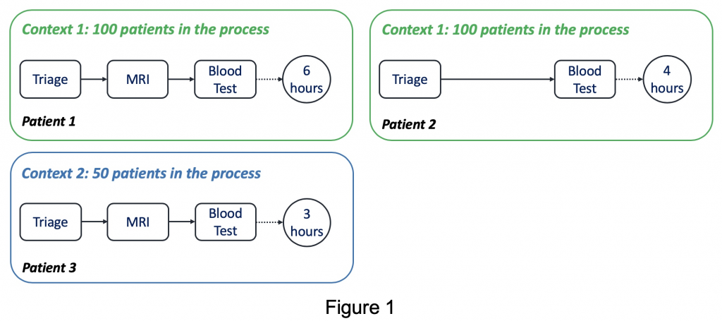
Assume that we are interested in building a model to find the correlation between the activity records that a patient went through in the past (predictor-case property) and the number of ongoing patients in the process (predictor-context of a business process) and the remaining time (predictand). In context1 with 100 ongoing patients, Patient1 went through Triage, MRI, Blood Test in the past, and the remaining time was 6 hours. On the other hand, Patient2 was in the same context as Patient1 while skipping MRI compared to Patient1, and the remaining time was 4 hours. From these observations, we are able to find that the existence of an MRI operation is positively correlated to the remaining time (possibly due to the following additional operations like MRI evaluation, etc.).
Patient3 was in context2 with 50 ongoing patients and went through the same activities as Patient1, but the remaining time was 3 hours. Based on this, we can conclude that the number of ongoing patients in the process is negatively correlated to the remaining time. The discovered correlations can be used to predict the remaining times of any given running instances with its values of predictors.
2. Resource allocation in business process
Resource allocation is to allocate appropriate resources to tasks at the correct time, which enables to improve productivity, balance resource usage, and reduce execution costs. Resource allocation in business process management shares commonalities with the Job Shop Scheduling Problem (JSSP). JSSP is to find the job sequences on machines to achieve a goal (e.g., minimizing makespans), while the machine sequence of the jobs is fixed.
A huge amount of approaches has been suggested to solve JSSP in the field of operations research. One of the promising approaches is dispatching rules due to its computing efficiency and robustness to uncertainty.
However, those techniques require parameters such as the release time, the processing time, and the sequence of operations of jobs. Indeed, in many cases of business processes, we have limited information that prohibits the deployment of them. For instance, in an emergency department of a hospital, we do not know when and why a patient would come into the department before the visit happens, clinical procedures of the patient, and the processing time taken for resources to finish an operation.
3. Prediction-based resources allocation
You may expect what comes next. Yes, we can exploit the techniques from predictive business process monitoring to deal with resource allocation in business processes where required parameters for scheduling are missing. To this end, first, we predict the relevant parameters (e.g., the subsequent activities of the patients and their processing times) and then utilize them to optimize resource allocation.
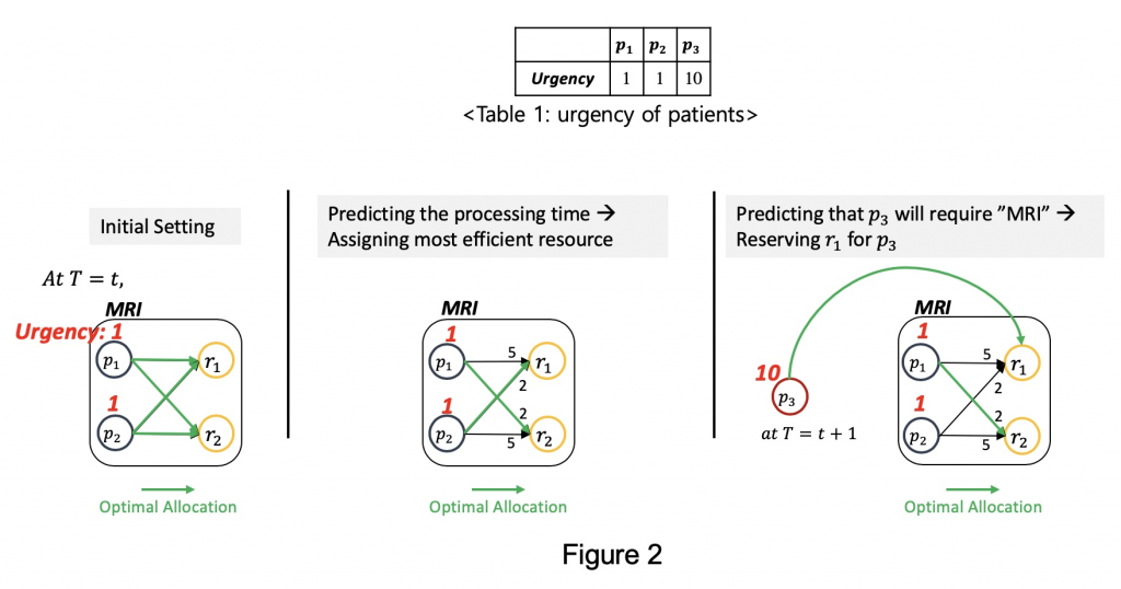
Suppose we optimize the resource allocation at time in MRI operation, as shown in Figure 2, with respect to the total weighted completion time. Note that we use the urgency of patients, described in Table 1, as weights. The higher the urgency of a patient is, the more weight he/she is assigned to. In other words, we want to assign resources to patients in a way that minimizes the processing time, and, at the same time, treat urgent patients earlier than others.
Let’s first consider the initial setting where we don’t have any information for resource allocation. In this case, there is no option but to randomly assign patients to resources. Next, suppose we have the information about processing time required for resources to treat different patients. In this case, we can assign the most efficient resource to each patient, i.e., p1 to r2 and p2 to r1. Finally, assume that we predict that an urgent patient, p3, is about to require MRI operation at time t+1. In this case, we can reserve a resource to wait for this patient since it is more efficient in terms of total weighted completion time, i.e., at t, p1 to r2 and at t+1, p3 to r1. To sum up, if we predict the processing time and the next activity of a patient, we can tremendously improve the scheduling performance.
Then, how can we solve it in an algorithmic way? For this, we formulate the resource allocation problem into minimum cost and maximum flow problem, where we aim at maximizing the number of flows while minimizing the cost of flows. This problem is solved in polynomial time by network simplex method, so the algorithm for resource allocation is.
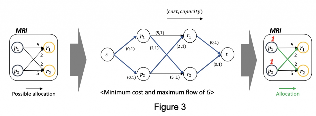
Figure 3 shows how we formulate it. Based on the parameters we predicted (the leftmost), we add source node and sink node . Besides, we annotate on each arc. The arcs coming from source node and to source node always has (0, 1), while cost of other arcs are designed to be proportional to the processing time. By applying network simplex method in this graph, we get the optimal resource allocations as depicted as green arcs in the rightmost.
For more information,
Check out slides of ICPM 2019
- G. Park and M. Song, “Prediction-based Resource Allocation using LSTM and Minimum Cost and Maximum Flow Algorithm”, 2019 International Conference on Process Mining (ICPM), Aachen, Germany, 2019, pp. 121-128.
PM4KNIME: a bridge between ProM and KNIME
This post is by Kefang Ding, Scientific Assistant in the Process And Data Science group at RWTH Aachen University. Contact her via email for further inquiries.
ProM is a scientific open-source platform for process mining techniques, which is popular among researchers. Many algorithms in process mining are implemented as ProM plugins. However, users interact with those plugins separately. It makes it difficult and time-consuming to conduct analyses which require multiple plugins or tests which require repeated execution of the same sequence of plugins.
Workflow management systems are software tools designed to create, perform and monitor a defined sequence of tasks. Among the current workflow management systems, KNIME is a free and open-source data analytics platform, which is implemented in Java but also allows for wrappers to run Java, Python, Perl and other frameworks.
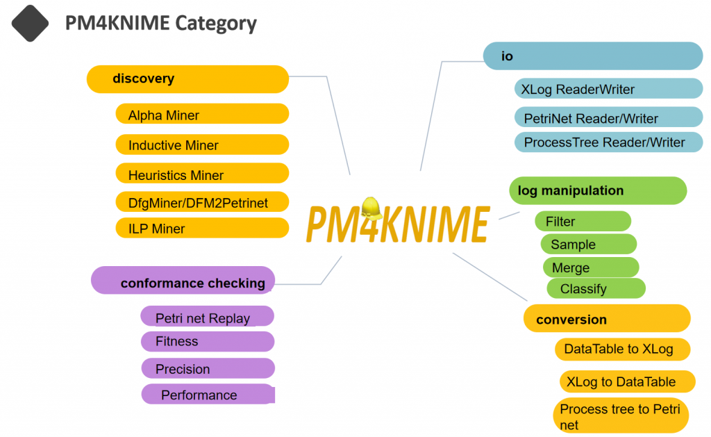
In order to overcome the drawbacks of ProM on workflow management, as well as to enable the use of process mining techniques in KNIME, we have developed a project called PM4KNIME. PM4KNIME integrates the ProcessMining tools from ProM into KNIME platform by wrapping ProM plugins as nodes in KNIME.
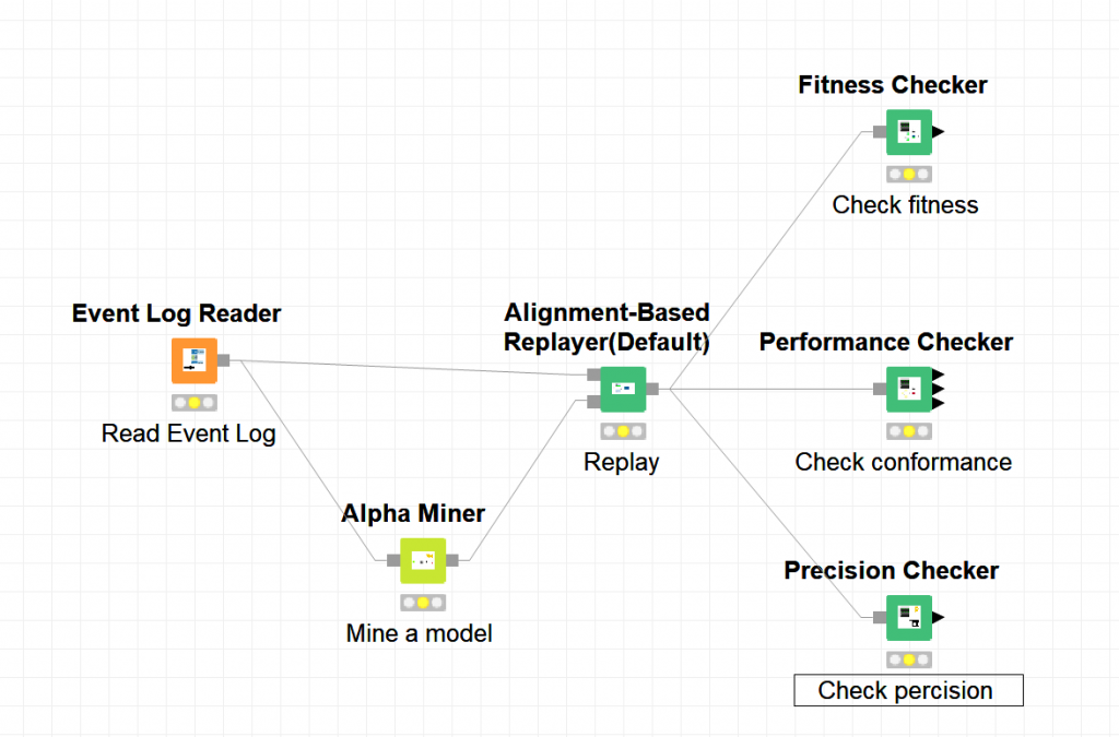
To conduct tasks in Process Mining with PM4KNIME, nodes are connected to compose a workflow. Then the workflow can be executed multiple times by one click. For example, to complete the task on checking the performance, fitness and precision of an event log and a Petri net, the workflow in KNIME is shown below.
With the same tasks, compared to ProM, PM4KNIME allows an easy configuration with less interaction, easy reuse and sharing with the workflow.
The current PM4KNIME extensions implement the nodes for frequent-used process mining techniques. The PM4KNIME taxonomy is listed below.
Click on the link (https://github.com/pm4knime/pm4knime-document/wiki) to learn more about PM4KNIME! If you are interested in PM4KNIME, please contact us with kefang.ding@pads.rwth-aachen.de
Efficient Construction of Behavior Graphs for Uncertain Event Data
This post is by Marco Pegoraro, Scientific Assistant in the Process And Data Science group at RWTH Aachen University. Contact him via email for further inquiries.
In previous posts on this blog, we talked about uncertainty in process mining, both in the context of conformance checking and process discovery. In an uncertain process trace, the attributes of an event are not recorded as a precise value but as a range or a set of alternatives.
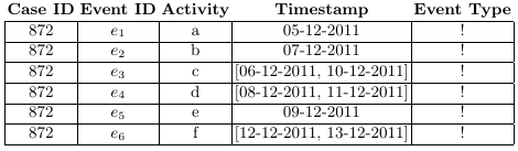
If we consider the case of timestamps represented as ranges, the total order usually present among events in a trace is lost; time relationships exist in a partial order instead, where the order between events that have overlapping timestamps is undefined. The directed acyclic graph that graphically represents this partial order is called a behavior graph.
A straightforward way to obtain a behavior graph is to check all pairs of events, connecting the ones that have a well-defined time relationship, then perform a transitive reduction to remove unnecessary edges. This runs in a cubic time with respect to the number of events. In the paper “Efficient Construction of Behavior Graphs for Uncertain Event Data” (Pegoraro, Uysal, van der Aalst) we present a method to build behavior graphs in quadratic time, leading to a more efficient analysis of uncertain data in process mining.
Beyond Precision and Recall: Using Earth Mover’s Distance & Stochastics
This post is by Prof. Dr. Wil van der Aalst, Chairholder in the Process And Data Science group at RWTH Aachen University. Contact him via email for further inquiries.
Conformance checking aims to uncover differences between a process model and an event log. Initially, process mining focused on discovering process models from event data, but in recent years, the use and importance of conformance checking increased. Many conformance checking techniques and measures have been proposed. Typically, these take into account the frequencies of traces in the event log, but do not consider the probabilities of these traces in the model. This asymmetry leads to various complications. A novel way to approach this, is to assume probabilities and subsequently use the Earth Movers’ Distance (EMD) between stochastic languages representing models and event logs.
The Earth Movers’ Distance (EMD) provides and simple and intuitive conformance notion. The typical problems related to precision vanish immediately! Moreover, the approach is extensible to other perspectives (including time and resources) and can also be applied to concept drift detection and comparative process mining. This blog post summarizes part of my presentation given on 19-11-2019 in the weekly PADS Seminar Series (slides are attached at the bottom of the page).
What is the problem?
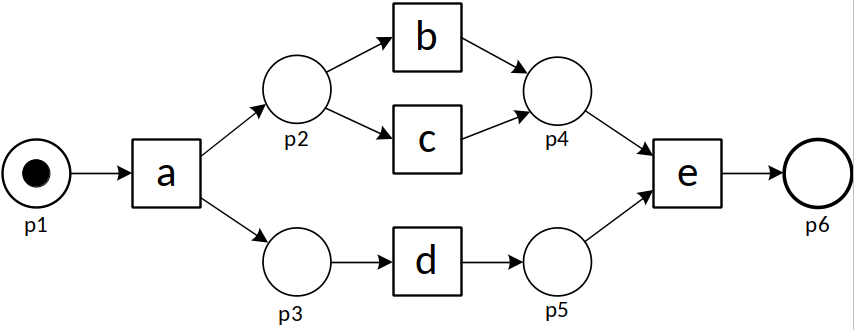
To explain the problem, let us consider the following process model and five event logs (L1 – L5).
| L1 | = [〈a,b,d,e〉490,〈a,d,b,e〉490,〈a,c,d,e〉10,〈a,d,c,e〉10] |
| L2 | = [〈a,b,d,e〉245,〈a,d,b,e〉245,〈a,c,d,e〉5,〈a,d,c,e〉5,〈a,b,e〉500] |
| L3 | = [〈a,b,d,e〉489,〈a,d,b,e〉489,〈a,c,d,e〉10,〈a,d,c,e〉10,〈a,b,e〉2] |
| L4 | = [〈a,b,d,e〉500,〈a,d,b,e〉500] |
| L5 | = [〈a,c,d,e〉500,〈a,d,c,e〉500] |
Each trace in L1 matches a trace of the model and vice versa. Hence, all existing recall and precision measures tend to give a high score (i.e., good conformance). Half of the traces in L2 do not fit the model (〈a,b,e〉is impossible according to the model, but occurs 500 times). Hence, all existing recall measures will report a low recall score for L2. However, these measures will report a high score for recall when L3 is considered. The reason is that in L3, 99.8% of the traces are fitting (〈a,b,e〉occurs only twice). Existing recall measures tend to give high scores when L4 and L5 are considered since the model can reproduce all traces observed. However, both L4 and L5 are only covering two of the four traces allowed by the process model. Hence, existing precision measures tend to give a lower score for L4 and L5. Moreover, due to symmetry, there is no reason to consider L4 and L5 to be different from a precision point of view.
The above analysis of existing recall measures shows that frequencies matter. L2 and L3 have the same sets of traces, but 50% of the traces of L2 are fitting and 99.8% of the traces of L3 are fitting. Hence, most recall measures will consider L3 to conform much better than L2. The logical counterpart of frequencies in event logs are routing probabilities in process models. However, almost all existing measures ignore such routing probabilities. This leads to an asymmetry.
Therefore, we argue that also probabilities matter.
Probabilities matter!
We start by adding probabilities to the process model introduced before.
The numbers attached to transitions can be interpreted as weights. The probability of trace〈a,d,b,e〉is 0.5×0.98 = 0.49, the probability of trace〈a,d,c,e〉is 0.5 ×0.02 = 0.01, etc. Hence, the model describes a so-called stochastic language:
| M | = [〈a,b,d,e〉0.49,〈a,d,b,e〉0.49,〈a,c,d,e〉0.01,〈a,d,c,e〉0.01] |
Similarly, we can convert trace frequencies into probabilities:
| L1 | = [〈a,b,d,e〉0.49,〈a,d,b,e〉0.49,〈a,c,d,e〉0.01,〈a,d,c,e〉0.01] |
| L2 | = [〈a,b,d,e〉0.245,〈a,d,b,e〉0.245,〈a,c,d,e〉0.005,〈a,d,c,e〉0.005,〈a,b,e〉0.5] |
| L3 | = [〈a,b,d,e〉0.489,〈a,d,b,e〉0.489,〈a,c,d,e〉0.01,〈a,d,c,e〉0.01,〈a,b,e〉0.002] |
| L4 | = [〈a,b,d,e〉0.5,〈a,d,b,e〉0.5] |
| L5 | = [〈a,c,d,e〉0.5,〈a,d,c,e〉0.5] |
By converting event logs and process models to stochastic languages, conformance is reduced to the problem of comparing stochastic languages.
Consider model M and the five event logs L1, L2, L3, L4, and L5. Obviously, L3 is closer to M than L2. Similarly, L4 is closer to M than L5. We propose to use the so-called Earth Mover’s Distance (EMD) to compare stochastic languages. If the probabilities of traces are considered as piles of sand, then EMD is the minimum cost of moving the sand from one distribution to another. EMD requires a distance notion. For our Earth Movers’ Stochastic Conformance notion, we provided several distance notions, e.g., the normalized edit distance between two traces.
Earth Movers’ Stochastic Conformance
If we assume the normalized edit distance between traces, then the EMD distance is a number between 0 (identical, i.e., fully conforming) and 1 (worst possible conformance). For our model M and logs L1,L2, …, L5 we find the following distances: 0 for L1, 0.125 for L2, 0.0005 for L3, 0.005 for L4, and 0.245 for L5. Note that distance is the inverse of similarity, i.e., for model M and logs L1,L2, …, L5 we find the following Earth Movers’ Stochastic Conformance similarity measures: 1 for L1, 0.875 for L2, 0.9995 for L3, 0.995 for L4, and 0.755 for L5. Hence, given M, L1 has the best conformance, L3 is much better than L2, and L4 is much better than L5. This matches our intuition, e.g., L5 does not have any executions of b although, according to the model, b should be executed for 98% of cases. Note that there is just one conformance measure and not two separate measures for recall and precision. This makes sense considering that increasing the probability of one trace should coincide with lowering the probabilities of other traces.
Just the starting point!
The approach is very promising and has been implemented in ProM. This was mostly done by Sander Leemans from QUT. Next, to these conformance measures, we also defined various types of diagnostics to identify conformance problems in both log and model. In addition, challenges related to infinite loops, duplicate activities, and silent activities have been addressed. Recently, also Tobias Brockhoff joined the team and is focusing on using the EMD notion to concept drift, i.e., detecting when and how process change. Moreover, he also extended the above techniques with time. This allows us to see how performance is changing. These techniques are being applied in the Internet of Production (IoP) Cluster of Excellence at RWTH. The work of Tobias can be used to find and diagnose performance problems and uncover changes in routing and delays in production systems.
Learn More?
Check out the slides of the PADS Seminar Series.
- S.J.J. Leemans, A.F. Syring, and W.M.P. van der Aalst. Earth Movers’ Stochastic Conformance Checking. In T.T. Hildebrandt, B.F. van Dongen, M. Röglinger, and J. Mendling, editors, Business Process Management Forum (BPM Forum 2019), volume 360 of Lecture Notes in Business Information Processing, pages 127-143. Springer-Verlag, Berlin, 2019.
- W.M.P. van der Aalst, A. Adriansyah, and B. van Dongen. Replaying History on Process Models for Conformance Checking and Performance Analysis. WIREs Data Mining and Knowledge Discovery, 2(2):182-192, 2012.