Prediction-based recommendation in process mining
This post is by Gyunam Park, Scientific Assistant in the Process And Data Science group at RWTH Aachen University. Contact him via email for further inquiries.
Process mining has provided effective techniques to extract in-depth insights into business processes such as process discovery, conformance checking, and enhancement. Nowadays, with the increasing availability of real-time data and sufficient computing power, practitioners are more interested in forward looking techniques whose insights can be used to improve performances and mitigate risks of running process instances.
Research on these forward looking techniques has been actively done in the field of process mining. Predictive business process monitoring is one of those approaches, whose aim is to improve business processes by offering timely information (e.g., remaining time of running instances) that enables proactive and corrective actions.
However, these techniques do not suggest how the predictions are exploited to improve business processes, leaving it up to the subjective judgment of practitioners. The transformation from predictions to concrete actions remain as missing link to achieve the goal of process improvement.
A recent paper, “Prediction-based Resource Allocation using LSTM and Minimum Cost and Maximum Flow Algorithm”, demonstrate an effort to connect the missing link between the predictive insights to concrete recommendations, which enables process improvement. In the paper, authors exploit the prediction results from predictive business process monitoring techniques to recommend optimal resource allocations in business processes.
In the following, I will explain 1) Predictive business process monitoring, 2) Resource allocation in business process, and 3) Prediction-based recommendation (specifically for resource allocation).
1. Predictive business process monitoring
Predictive business process monitoring techniques provide insightful predictions on running instances in business processes. The techniques can be divided into several categories depending on the type of values they aim to predict. The primary types of predictions include
- remaining time (i.e., how much time is left to complete a case),
- risk probability (i.e., how probable it is for a case to fail at the end),
- next event (i.e., the property of the next event (e.g., next activity) of a case).
How can we predict those values? There exist several different approaches, but in a simple way, we can think of them as finding a correlation between features (i.e., predictors) and the target values (i.e., predictand).
There are mainly two types of predictors that can be used to describe predictand. The first type is the case property, which indicates the case attributes (e.g., the membership of a customer) or the event attributes that are related to the case (e.g., the previous treatments a customer went through in the process). The second type is the context of a business process, which describes the status of the process at the time predictions are made (e.g., the total number of ongoing cases in the process and the total number of resources in the process, etc.).
Let’s have a look at the example showing how we derive the correlation between predictors and predictand.
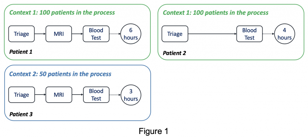
Assume that we are interested in building a model to find the correlation between the activity records that a patient went through in the past (predictor-case property) and the number of ongoing patients in the process (predictor-context of a business process) and the remaining time (predictand). In context1 with 100 ongoing patients, Patient1 went through Triage, MRI, Blood Test in the past, and the remaining time was 6 hours. On the other hand, Patient2 was in the same context as Patient1 while skipping MRI compared to Patient1, and the remaining time was 4 hours. From these observations, we are able to find that the existence of an MRI operation is positively correlated to the remaining time (possibly due to the following additional operations like MRI evaluation, etc.).
Patient3 was in context2 with 50 ongoing patients and went through the same activities as Patient1, but the remaining time was 3 hours. Based on this, we can conclude that the number of ongoing patients in the process is negatively correlated to the remaining time. The discovered correlations can be used to predict the remaining times of any given running instances with its values of predictors.
2. Resource allocation in business process
Resource allocation is to allocate appropriate resources to tasks at the correct time, which enables to improve productivity, balance resource usage, and reduce execution costs. Resource allocation in business process management shares commonalities with the Job Shop Scheduling Problem (JSSP). JSSP is to find the job sequences on machines to achieve a goal (e.g., minimizing makespans), while the machine sequence of the jobs is fixed.
A huge amount of approaches has been suggested to solve JSSP in the field of operations research. One of the promising approaches is dispatching rules due to its computing efficiency and robustness to uncertainty.
However, those techniques require parameters such as the release time, the processing time, and the sequence of operations of jobs. Indeed, in many cases of business processes, we have limited information that prohibits the deployment of them. For instance, in an emergency department of a hospital, we do not know when and why a patient would come into the department before the visit happens, clinical procedures of the patient, and the processing time taken for resources to finish an operation.
3. Prediction-based resources allocation
You may expect what comes next. Yes, we can exploit the techniques from predictive business process monitoring to deal with resource allocation in business processes where required parameters for scheduling are missing. To this end, first, we predict the relevant parameters (e.g., the subsequent activities of the patients and their processing times) and then utilize them to optimize resource allocation.
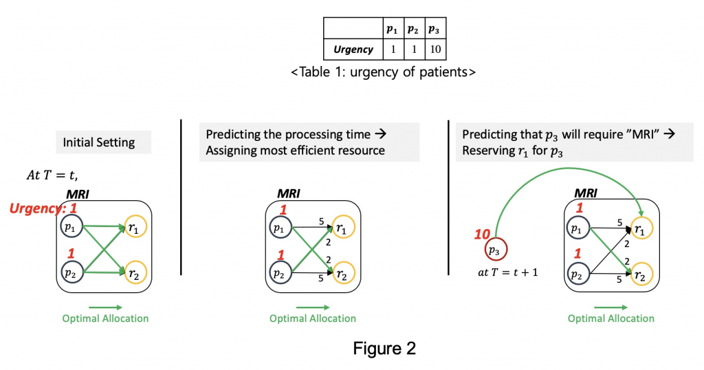
Suppose we optimize the resource allocation at time in MRI operation, as shown in Figure 2, with respect to the total weighted completion time. Note that we use the urgency of patients, described in Table 1, as weights. The higher the urgency of a patient is, the more weight he/she is assigned to. In other words, we want to assign resources to patients in a way that minimizes the processing time, and, at the same time, treat urgent patients earlier than others.
Let’s first consider the initial setting where we don’t have any information for resource allocation. In this case, there is no option but to randomly assign patients to resources. Next, suppose we have the information about processing time required for resources to treat different patients. In this case, we can assign the most efficient resource to each patient, i.e., p1 to r2 and p2 to r1. Finally, assume that we predict that an urgent patient, p3, is about to require MRI operation at time t+1. In this case, we can reserve a resource to wait for this patient since it is more efficient in terms of total weighted completion time, i.e., at t, p1 to r2 and at t+1, p3 to r1. To sum up, if we predict the processing time and the next activity of a patient, we can tremendously improve the scheduling performance.
Then, how can we solve it in an algorithmic way? For this, we formulate the resource allocation problem into minimum cost and maximum flow problem, where we aim at maximizing the number of flows while minimizing the cost of flows. This problem is solved in polynomial time by network simplex method, so the algorithm for resource allocation is.
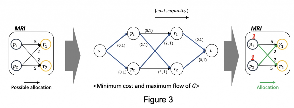
Figure 3 shows how we formulate it. Based on the parameters we predicted (the leftmost), we add source node and sink node . Besides, we annotate on each arc. The arcs coming from source node and to source node always has (0, 1), while cost of other arcs are designed to be proportional to the processing time. By applying network simplex method in this graph, we get the optimal resource allocations as depicted as green arcs in the rightmost.
For more information,
Check out slides of ICPM 2019
- G. Park and M. Song, “Prediction-based Resource Allocation using LSTM and Minimum Cost and Maximum Flow Algorithm”, 2019 International Conference on Process Mining (ICPM), Aachen, Germany, 2019, pp. 121-128.
PM4KNIME: a bridge between ProM and KNIME
This post is by Kefang Ding, Scientific Assistant in the Process And Data Science group at RWTH Aachen University. Contact her via email for further inquiries.
ProM is a scientific open-source platform for process mining techniques, which is popular among researchers. Many algorithms in process mining are implemented as ProM plugins. However, users interact with those plugins separately. It makes it difficult and time-consuming to conduct analyses which require multiple plugins or tests which require repeated execution of the same sequence of plugins.
Workflow management systems are software tools designed to create, perform and monitor a defined sequence of tasks. Among the current workflow management systems, KNIME is a free and open-source data analytics platform, which is implemented in Java but also allows for wrappers to run Java, Python, Perl and other frameworks.
In order to overcome the drawbacks of ProM on workflow management, as well as to enable the use of process mining techniques in KNIME, we have developed a project called PM4KNIME. PM4KNIME integrates the ProcessMining tools from ProM into KNIME platform by wrapping ProM plugins as nodes in KNIME.
To conduct tasks in Process Mining with PM4KNIME, nodes are connected to compose a workflow. Then the workflow can be executed multiple times by one click. For example, to complete the task on checking the performance, fitness and precision of an event log and a Petri net, the workflow in KNIME is shown below.
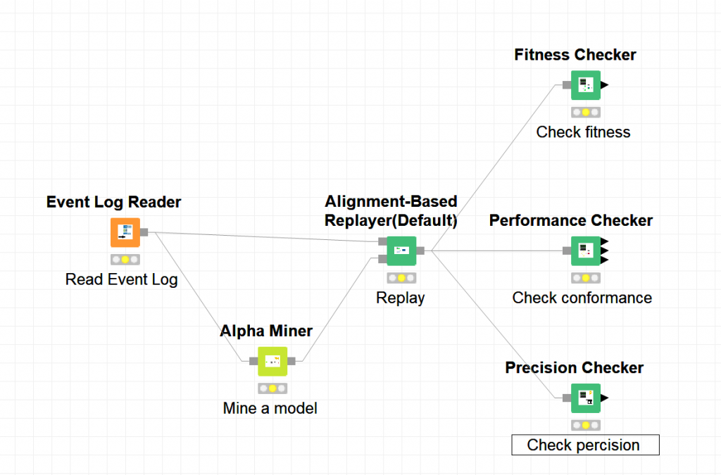
With the same tasks, compared to ProM, PM4KNIME allows an easy configuration with less interaction, easy reuse and sharing with the workflow.
The current PM4KNIME extensions implement the nodes for frequent-used process mining techniques. The PM4KNIME taxonomy is listed below.
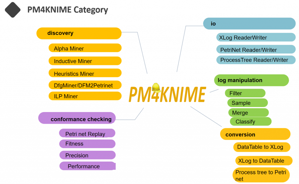
Click on the link (https://github.com/pm4knime/pm4knime-document/wiki) to learn more about PM4KNIME! If you are interested in PM4KNIME, please contact us with kefang.ding@pads.rwth-aachen.de
Efficient Construction of Behavior Graphs for Uncertain Event Data
This post is by Marco Pegoraro, Scientific Assistant in the Process And Data Science group at RWTH Aachen University. Contact him via email for further inquiries.
In previous posts on this blog, we talked about uncertainty in process mining, both in the context of conformance checking and process discovery. In an uncertain process trace, the attributes of an event are not recorded as a precise value but as a range or a set of alternatives.

If we consider the case of timestamps represented as ranges, the total order usually present among events in a trace is lost; time relationships exist in a partial order instead, where the order between events that have overlapping timestamps is undefined. The directed acyclic graph that graphically represents this partial order is called a behavior graph.
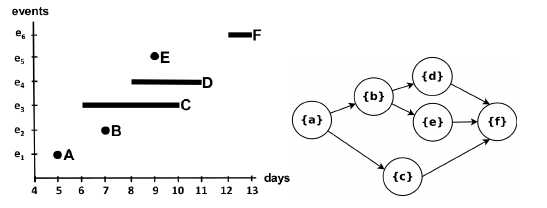
A straightforward way to obtain a behavior graph is to check all pairs of events, connecting the ones that have a well-defined time relationship, then perform a transitive reduction to remove unnecessary edges. This runs in a cubic time with respect to the number of events. In the paper “Efficient Construction of Behavior Graphs for Uncertain Event Data” (Pegoraro, Uysal, van der Aalst) we present a method to build behavior graphs in quadratic time, leading to a more efficient analysis of uncertain data in process mining.
Beyond Precision and Recall: Using Earth Mover’s Distance & Stochastics
This post is by Prof. Dr. Wil van der Aalst, Chairholder in the Process And Data Science group at RWTH Aachen University. Contact him via email for further inquiries.
Conformance checking aims to uncover differences between a process model and an event log. Initially, process mining focused on discovering process models from event data, but in recent years, the use and importance of conformance checking increased. Many conformance checking techniques and measures have been proposed. Typically, these take into account the frequencies of traces in the event log, but do not consider the probabilities of these traces in the model. This asymmetry leads to various complications. A novel way to approach this, is to assume probabilities and subsequently use the Earth Movers’ Distance (EMD) between stochastic languages representing models and event logs.
The Earth Movers’ Distance (EMD) provides and simple and intuitive conformance notion. The typical problems related to precision vanish immediately! Moreover, the approach is extensible to other perspectives (including time and resources) and can also be applied to concept drift detection and comparative process mining. This blog post summarizes part of my presentation given on 19-11-2019 in the weekly PADS Seminar Series (slides are attached at the bottom of the page).
What is the problem?
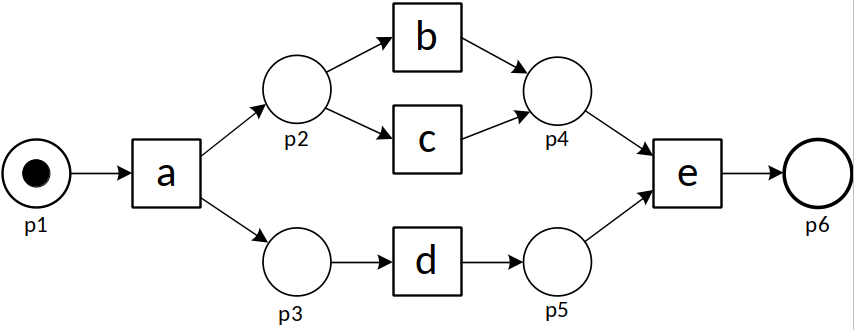
To explain the problem, let us consider the following process model and five event logs (L1 – L5).
| L1 | = [〈a,b,d,e〉490,〈a,d,b,e〉490,〈a,c,d,e〉10,〈a,d,c,e〉10] |
| L2 | = [〈a,b,d,e〉245,〈a,d,b,e〉245,〈a,c,d,e〉5,〈a,d,c,e〉5,〈a,b,e〉500] |
| L3 | = [〈a,b,d,e〉489,〈a,d,b,e〉489,〈a,c,d,e〉10,〈a,d,c,e〉10,〈a,b,e〉2] |
| L4 | = [〈a,b,d,e〉500,〈a,d,b,e〉500] |
| L5 | = [〈a,c,d,e〉500,〈a,d,c,e〉500] |
Each trace in L1 matches a trace of the model and vice versa. Hence, all existing recall and precision measures tend to give a high score (i.e., good conformance). Half of the traces in L2 do not fit the model (〈a,b,e〉is impossible according to the model, but occurs 500 times). Hence, all existing recall measures will report a low recall score for L2. However, these measures will report a high score for recall when L3 is considered. The reason is that in L3, 99.8% of the traces are fitting (〈a,b,e〉occurs only twice). Existing recall measures tend to give high scores when L4 and L5 are considered since the model can reproduce all traces observed. However, both L4 and L5 are only covering two of the four traces allowed by the process model. Hence, existing precision measures tend to give a lower score for L4 and L5. Moreover, due to symmetry, there is no reason to consider L4 and L5 to be different from a precision point of view.
The above analysis of existing recall measures shows that frequencies matter. L2 and L3 have the same sets of traces, but 50% of the traces of L2 are fitting and 99.8% of the traces of L3 are fitting. Hence, most recall measures will consider L3 to conform much better than L2. The logical counterpart of frequencies in event logs are routing probabilities in process models. However, almost all existing measures ignore such routing probabilities. This leads to an asymmetry.
Therefore, we argue that also probabilities matter.
Probabilities matter!
We start by adding probabilities to the process model introduced before.
The numbers attached to transitions can be interpreted as weights. The probability of trace〈a,d,b,e〉is 0.5×0.98 = 0.49, the probability of trace〈a,d,c,e〉is 0.5 ×0.02 = 0.01, etc. Hence, the model describes a so-called stochastic language:
| M | = [〈a,b,d,e〉0.49,〈a,d,b,e〉0.49,〈a,c,d,e〉0.01,〈a,d,c,e〉0.01] |
Similarly, we can convert trace frequencies into probabilities:
| L1 | = [〈a,b,d,e〉0.49,〈a,d,b,e〉0.49,〈a,c,d,e〉0.01,〈a,d,c,e〉0.01] |
| L2 | = [〈a,b,d,e〉0.245,〈a,d,b,e〉0.245,〈a,c,d,e〉0.005,〈a,d,c,e〉0.005,〈a,b,e〉0.5] |
| L3 | = [〈a,b,d,e〉0.489,〈a,d,b,e〉0.489,〈a,c,d,e〉0.01,〈a,d,c,e〉0.01,〈a,b,e〉0.002] |
| L4 | = [〈a,b,d,e〉0.5,〈a,d,b,e〉0.5] |
| L5 | = [〈a,c,d,e〉0.5,〈a,d,c,e〉0.5] |
By converting event logs and process models to stochastic languages, conformance is reduced to the problem of comparing stochastic languages.
Consider model M and the five event logs L1, L2, L3, L4, and L5. Obviously, L3 is closer to M than L2. Similarly, L4 is closer to M than L5. We propose to use the so-called Earth Mover’s Distance (EMD) to compare stochastic languages. If the probabilities of traces are considered as piles of sand, then EMD is the minimum cost of moving the sand from one distribution to another. EMD requires a distance notion. For our Earth Movers’ Stochastic Conformance notion, we provided several distance notions, e.g., the normalized edit distance between two traces.
Earth Movers’ Stochastic Conformance
If we assume the normalized edit distance between traces, then the EMD distance is a number between 0 (identical, i.e., fully conforming) and 1 (worst possible conformance). For our model M and logs L1,L2, …, L5 we find the following distances: 0 for L1, 0.125 for L2, 0.0005 for L3, 0.005 for L4, and 0.245 for L5. Note that distance is the inverse of similarity, i.e., for model M and logs L1,L2, …, L5 we find the following Earth Movers’ Stochastic Conformance similarity measures: 1 for L1, 0.875 for L2, 0.9995 for L3, 0.995 for L4, and 0.755 for L5. Hence, given M, L1 has the best conformance, L3 is much better than L2, and L4 is much better than L5. This matches our intuition, e.g., L5 does not have any executions of b although, according to the model, b should be executed for 98% of cases. Note that there is just one conformance measure and not two separate measures for recall and precision. This makes sense considering that increasing the probability of one trace should coincide with lowering the probabilities of other traces.
Just the starting point!
The approach is very promising and has been implemented in ProM. This was mostly done by Sander Leemans from QUT. Next, to these conformance measures, we also defined various types of diagnostics to identify conformance problems in both log and model. In addition, challenges related to infinite loops, duplicate activities, and silent activities have been addressed. Recently, also Tobias Brockhoff joined the team and is focusing on using the EMD notion to concept drift, i.e., detecting when and how process change. Moreover, he also extended the above techniques with time. This allows us to see how performance is changing. These techniques are being applied in the Internet of Production (IoP) Cluster of Excellence at RWTH. The work of Tobias can be used to find and diagnose performance problems and uncover changes in routing and delays in production systems.
Learn More?
Check out the slides of the PADS Seminar Series.
- S.J.J. Leemans, A.F. Syring, and W.M.P. van der Aalst. Earth Movers’ Stochastic Conformance Checking. In T.T. Hildebrandt, B.F. van Dongen, M. Röglinger, and J. Mendling, editors, Business Process Management Forum (BPM Forum 2019), volume 360 of Lecture Notes in Business Information Processing, pages 127-143. Springer-Verlag, Berlin, 2019.
- W.M.P. van der Aalst, A. Adriansyah, and B. van Dongen. Replaying History on Process Models for Conformance Checking and Performance Analysis. WIREs Data Mining and Knowledge Discovery, 2(2):182-192, 2012.
MicroPM4Py – Process Mining in Resource-Constrained Environments
This post is by Alessandro Berti, Software Engineer in the Process And Data Science group at RWTH Aachen University. Contact him via email for further inquiries.
Process mining is a branch of data science that includes a wide set of different techniques for automated process discovery, compliance/conformance checking, process simulation and prediction. The tools support for process mining has developed in the recent years in different directions: standalone tools, libraries for the most known programming languages, cloud solutions that store and analyze event data. All of these require the support of different standards, numeric calculus and optimization techniques, visualizations. Examples are the XES standard (XML) for the storage of event logs, the support of Petri nets and their importing/exporting from PNML (XML) files, the inclusion of LP/ILP solvers for process discovery (ILP-based process discovery) and conformance checking (A* alignments).
The inclusion of a vast set of functionalities in the more advanced tools/libraries (like ProM 6.x or PM4Py) has therefore led to an uncontrollable growth in the amount of memory required to run the tool/library. As per now, simply opening ProM 6.9 requires more than 650 MB of RAM, and importing PM4Py along with its dependencies requires more than 80 MB of RAM. On the other hand, cloud solutions such as the Celonis IBC or MyInvenio require an active Internet connection for the transmission of event data and the delivery of process mining analysis/dashboards.
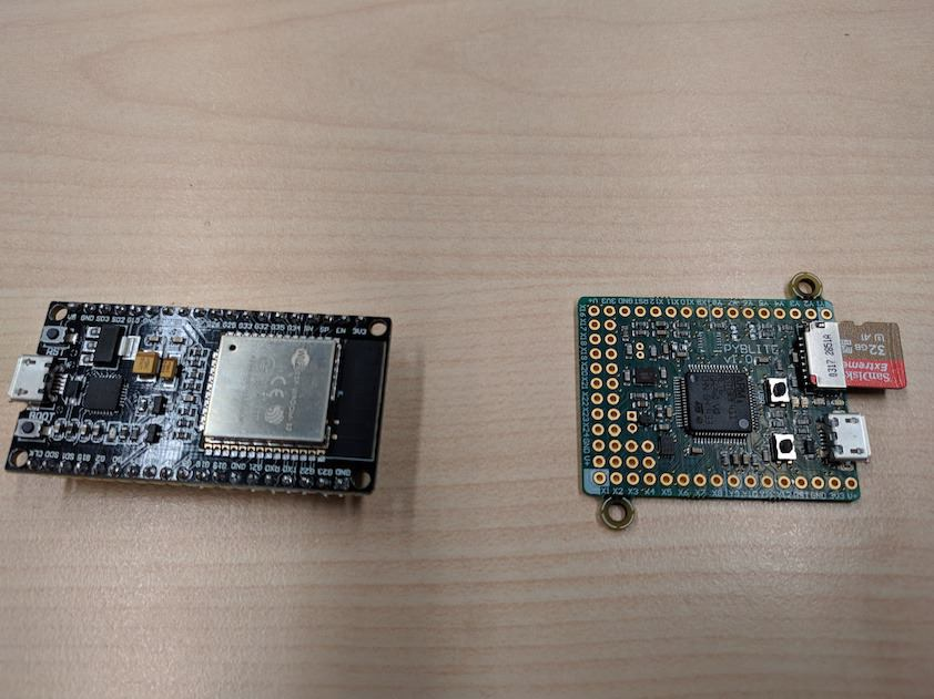
This cuts the possibility to apply process mining on the most numerous class of computers in the world: the microcontrollers. As example, a modern car contains from 30 to 70 microcontrollers. Microcontrollers are usually adopted to control the operational status of a system (for example, the acceleration, temperature, magnetic field, humidity). For minimizing idle/light sleep power consumption, these come with a very limited amount of RAM (usually from 32 KB to 512 KB) and a very low power CPU (examples are the Cortex M0/M4/M7 CPUs for microcontrollers). Applying existing process mining tools/libraries on these is simply impossible.
Hence, a new library (MicroPM4Py) is being developed in the MicroPython language (www.micropython.org), that is a complete reimplementation for microcontrollers of a basic set of features of Python 3.4. The aim of the MicroPython language is not being faster than the normal Python (indeed, Python is much faster than MicroPython for the same script) but to minimize the memory footprint of the application. The goal of MicroPM4Py is to enable some process mining features directly at the microcontroller level:
- Full support for Petri nets without invisible transitions: a memory-efficient data structure is deployed that supports the semantics of a Petri net, the verification of the fitness of a trace, PNML importing/exporting.
- Basic support (A1 import; A1 export) for the XES standard for event logs: the traces can be loaded from the XES event log with different modalities (full DFG; distinct variants; full list of traces in memory; iterator trace by trace).
- Basic support for importing/exporting logs in the CSV format.
- Basic support for process discovery (discovery of a DFG, DFG mining, Alpha Miner algorithm) on top of XES/CSV event logs
- Generation of the DOT (Graphviz) visualization of a DFG / Petri net.
All the data structures have been optimized in order to minimize the memory consumption. As example, the following table estimates the RAM occupation (in bytes) of the three log structures in MicroPM4Py reading the DFG from the XES; reading the variants; reading all the traces from the log. Generally, the numbers are competitive and among the most efficient XES importers ever done (remind the limitation: only the case ID and the activity is read).
| Log name | DFG obj size | Variants obj size | Loaded log obj size |
| running-example | 3200 | 1568 | 2016 |
| receipt | 17112 | 22072 | 213352 |
| roadtraffic | 10696 | 37984 | 19392280 |
| LevelA1.xes | 6456 | 16368 | 154792 |
| BPIC17.xes | 29240 | 7528144 | 11474448 |
| BPIC15_4.xes | 453552 | 488200 | 587656 |
| BPIC17 – Offer log.xes | 3768 | 2992 | 6051880 |
| BPIC13_incidents.xes | 2696 | 380216 | 1333200 |
| BPIC15_3.xes | 600304 | 600312 | 743656 |
| BPIC15_1.xes | 541824 | 534216 | 652696 |
| BPIC15_5.xes | 555776 | 589688 | 703712 |
| BPIC12.xes | 20664 | 1819848 | 3352352 |
| BPIC13_closed_problems.xes | 2320 | 33504 | 226856 |
| BPIC15_2.xes | 551656 | 457496 | 531176 |
| BPIC13_open_problems.xes | 1872 | 16096 | 122672 |
The following table estimates the memory usage of an use case of MicroPM4Py: from a log, the DFG is obtained and the DFG mining technique is applied to obtain a Petri net. Then, an iterator is created on the log, in order to iterate over the single traces of the log. The memory usage of the MicroPM4Py module and data structure is then measured. The following aspects are taken into account (estimations were done on a X86-64 Debian 9 with Miniconda Python 3.7):
- The maximum size of the iterator+current trace (in bytes)
- The size of the DFG-mined Petri net (in bytes)
- The size of the MicroPM4Py Python module (in bytes)
- An estimated overapproximated size (16 KB) of a kernel + Micropython interpeter running on a microcontroller (in bytes)
The values are summed to get an estimation of the memory usage of the application for such use case, for several real-life logs. Except for the BPIC 2015 logs, the memory allocation is always under 128 KB! 🙂
| Log name | Max XES iterable size | DFG mining net size | MicroPM4Py module size | MicroPython size (est.max.) | MAX EST. SIZE |
| running-example | 2512 | 6384 | 20624 | 16384 | 45904 |
| receipt | 6312 | 27328 | 20624 | 16384 | 70648 |
| roadtraffic | 3416 | 18104 | 20624 | 16384 | 58528 |
| LevelA1.xes | 3656 | 9952 | 20624 | 16384 | 50616 |
| BPIC17.xes | 6664 | 41352 | 20624 | 16384 | 85024 |
| BPIC15_4.xes | 49560 | 757680 | 20624 | 16384 | 844248 |
| BPIC17 – Offer log.xes | 2392 | 6760 | 20624 | 16384 | 46160 |
| BPIC13_incidents.xes | 2696 | 5352 | 20624 | 16384 | 45056 |
| BPIC15_3.xes | 49912 | 1084872 | 20624 | 16384 | 1171792 |
| BPIC15_1.xes | 51592 | 993800 | 20624 | 16384 | 1082400 |
| BPIC15_5.xes | 54048 | 1027648 | 20624 | 16384 | 1118704 |
| BPIC12.xes | 6368 | 30744 | 20624 | 16384 | 74120 |
| BPIC13_closed_problems.xes | 2056 | 5160 | 20624 | 16384 | 44224 |
| BPIC15_2.xes | 54080 | 1012512 | 20624 | 16384 | 1103600 |
| BPIC13_open_problems.xes | 1864 | 4480 | 20624 | 16384 | 43352 |
While it is impossible on such level (microcontrollers) to support the wide set of features of other tools, it is still possible to apply some process mining algorithms on top of microcontrollers. MicroPM4Py can also be deployed on old workstations or other kinds of low-power computers (such as the Raspberry Pis).
As future work, the library will include some other process models (e.g. transition systems, NFA, continuous time markov chains).
Uncertanty in process mining: discovering models
This post is by Marco Pegoraro, Scientific Assistant in the Process And Data Science group at RWTH Aachen University. Contact him via email for further inquiries.
When applying process mining in real-life settings, the need to address anomalies in data recording when performing analyses is omnipresent. A number of such anomalies can be modeled by using the notion of uncertainty: uncertain event logs contain, alongside the event data, some attributes that describe a certain level of uncertainty affecting the data.
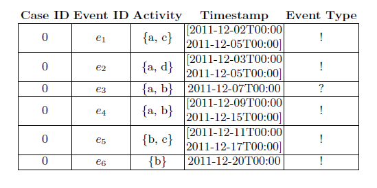
Uncertainty can be addressed by filtering out the affected events when it appears sporadically throughout an event log. Conversely, in situations where uncertainty affects a signifi cant fraction of an event log, fi ltering away uncertain events can lead to information loss such that analysis becomes very difficult. In this circumstance, it is important to deploy process mining techniques that allow to mine information also from the uncertain part of the process.
In the paper “Discovering Process Models from Uncertain Event Data” (Marco Pegoraro, Merih Seran Uysal, Wil M.P. van der Aalst) we present a methodology to obtain Uncertain Directly-Follows Graphs (UDFGs), models based on directed graphs that synthesize information about the uncertainty contained in the process. We then show how to convert UDFGs in models with execution semantics via fi ltering on uncertainty information and inductive mining.
Robotic Process Automation
This post is by Junxiong Gao, Scientific Assistant in the Process And Data Science group at RWTH Aachen University. Contact him via email for further inquiries.
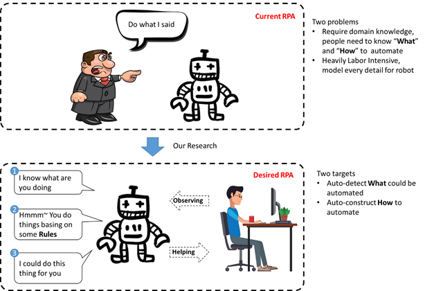
Robotic Process Automation (RPA) recently gained a lot of attention, both in industry and academia. RPA embodies a collection of tools and techniques that allow business owners to automate repetitive manual tasks. The intrinsic value of RPA is beyond dispute, e.g., automation reduces errors and costs and thus allows us to increase overall business process performance.
However, adoption of current-generation RPA tools requires a manual effort w.r.t. identification, elicitation and programming of the to-be-automated tasks. At the same time, several techniques exist that allow us to track the exact behavior of users, in great detail.
Therefore, in this line of research, we present a novel end-to-end structure design that allows for completely automated, algorithmic automation-rule deduction, on the basis of captured user behavior.
Uncertanty in process mining: finding bounds for conformance cost
This post is by Marco Pegoraro, Scientific Assistant in the Process And Data Science group at RWTH Aachen University. Contact him via email for further inquiries.
Let’s consider the analysis of a specific class of event logs: the logs that contain uncertain event data. Uncertain events are recordings of executions of specific activities in a process which are enclosed with an indication of uncertainty in the event attributes. Specifically, let’s consider the case where the attributes of an event are not recorded as a precise value but as a range or a set of alternatives. In the case of the common control-flow attributes of an event log, the case id and activity are represented by a set of alternatives, and the timestamp as a range.
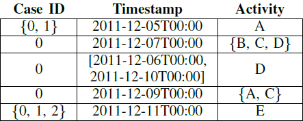
We can think of this uncertain trace as a set of “classic” traces obtained by every possible choices of the values for the attributes; this is called the realization set.
In the paper “Mining Uncertain Event Data in Process Mining“, published on the first International Conference on Process Mining (ICPM), we laid down a taxonomy of possible kinds of uncertainty; we also explore an example of application, i.e. the computation of upper and lower bound for conformance cost of an uncertain trace against a reference process model. This is obtained by modeling a Petri net able to reproduce the behavior of an uncertain trace; this enables to compute the conformance exploiting a model-to-model comparison.
Responsible Process Mining (RPM) – Confidentiality
This post is by Majid Rafiei, Scientific Assistant in the Process And Data Science group at RWTH Aachen University. Contact him via email for further inquiries.
To gain novel and valuable insights into the actual processes executed within a company, process mining provides a variety of powerful data-driven analyses techniques ranging from automatically discovering process models to detecting and predicting bottlenecks, and process deviations.
On the one hand, recent breakthroughs in process mining resulted in powerful techniques, encouraging organizations and business owners to improve their processes through process mining. On the other hand, there are great concerns about the use of highly sensitive event data. Within an organization, it often suffices that analysts only see the aggregated process mining results without being able to inspect individual cases, events, and persons. When analysis is outsourced also the results need to be encrypted to avoid confidentiality problems.
Surprisingly, little research has been done toward security methods and encryption techniques for process mining. The PADS team presented a novel approach that allows us to hide confidential information in a controlled manner while ensuring that the desired process mining results can still be obtained. In the following you can find a simplified version of our proposed framework.
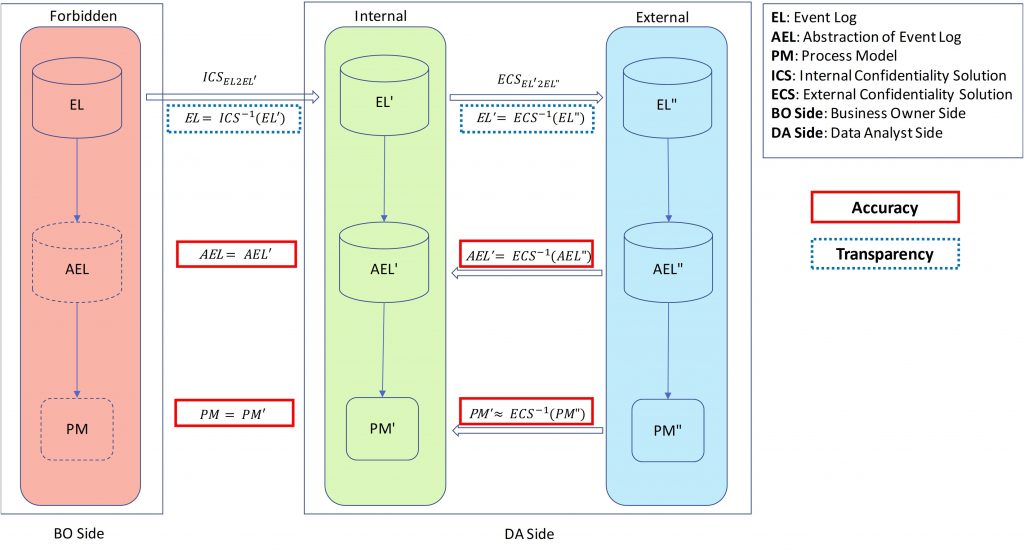
The paper which introduces this framework, and the connector method to preserve the sequence of activities securely has been selected as the best paper by SIMPDA 2018 (http://ceur-ws.org/Vol-2270/paper1.pdf). In this paper, we provide a sample solution for process discovery based on the above-mentioned framework.
Finding Complex Process-Structures by Exploiting the Token-game
This post is by Lisa Mannel, Scientific Assistant in the Process And Data Science group at RWTH Aachen University. Contact her via email for further inquiries.
Our paper „Finding Complex Process-Structures by Exploiting the Token-game“ has been accepted for publication by the 40th International Conference on Applications and Theory of Petri Nets and Concurrency.
In our paper we present a
novel approach to process discovery. In process discovery, the goal is to
find, for a given event log, the model describing the underlying process. While
process models can be represented in a variety of ways, in our paper we focus
on the representation by Petri nets. Using an approach inspired by
language-based regions, we start with a Petri net without any places, and then
insert the maximal set of places considered fitting with respect to the
behavior described by the log. Traversing and evaluating the whole set of all
possible places is not feasible, since their number is exponential in the
number of activities. Therefore, we propose a strategy to drastically prune
this search space to a small number of candidates, while still ensuring that
all fitting places are found. This allows us to derive complex model structures
that other discovery algorithms fail to discover. In contrast to traditional
region-based approaches this new technique can handle infrequent behavior and
therefore also noisy real-life event data. The drastic decrease of computation
time achieved by our pruning strategy, as well as our noise handling
capability, is demonstrated and evaluated by performing various experiments.
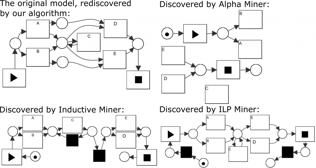
Figure 1: Consider the model shown in the upper left and assume L to be a complete log describing the behavior of this model. There exists a variety of discovery algorithms that are able to mine a process model based on L. As illustrated, the resulting Petri nets differ significantly between the algorithms. In particular, the places connecting A to D and B to E, which ensure that the first choice implies the second choice, are rarely discovered by existing algorithms.
You can download the full text here.

